Converting an 8 digit number to a Date in Google Sheets

Why the Date formula doesn't work as expected

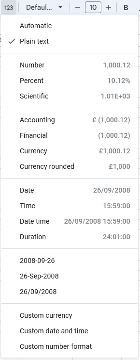
Recently I downloaded a list of transactions as a CSV file. The formatting for the date was an 8 digit number 20240826. No problem I thought, I can just convert it to a date by clicking 'more formats' and then choosing the correct date from custom date and time.

I clicked 1930-08-05 since this follows the same year, month and day order of the 8 digit number.

The result I got was not what I expected:

57316-01-26 🤔

Why are we getting this result?

The reason is that the Google Time Epoch began on 31 December 1899 00:00:00 (as opposed to the Unix Time Epoch, which is used by Javascript, which began on January 1, 1970 00:00:00). If you want to read a more detailed explanation this is a good reference.

You don't need to worry about why for the fix here because we're going to use Regex to break down the date into year, month and day. Then rebuild it again with the Date formula.

That sounds more complicated than it is. Let me walk you through it.

How to convert an 8 digit Date into a Date with separators using Regex

The solution

So we're starting with a cell with an 8 digit Date such as 20240826 and we went to end up with 26/08/2024 or 08/26/2024.

Here's how you do it.

1. Convert the current number to plain text

Select the cell with the 8 digit number in and convert it to plain text. We need to do this so the formula we're about to use in step 2 will work correctly.

2. Extracting the year with REGEXEXTRACT

Create a new column for the year and select the first cell, next to the 8 digit date.

Now we're going to use Regex to select the first 4 digits of the 8 digit string. We'll use the REGEXEXTRACT formular for this.

=REGEXEXTRACT(A2,"^\d{4}")

Place this into the first cell in the year column, make sure you're selecting the correct cell. In my case it is A2.

Here's what the Regex means:

• ^: Anchors the match to the start of the string.
• \d: Matches any digit.
• {4}: Specifies that the preceding \d should occur exactly four times.

So, this pattern will match the first four digits in a string of numbers, which in this case is our year.

Result:

3. Extracting the month

Now we're going to repeat the same steps, this time using a different pattern to get the month. Remember to change the target cell.

=REGEXEXTRACT(A2, "^\d{4}(\d{2})")

Here's what this pattern does:

• ^\d{4}: Matches the first four digits at the beginning of the string, as explained earlier.
• (\d{2}): This part captures the next two digits in a capturing group. The parentheses () are used to create a capturing group, and \d{2} matches exactly two digits.

4. Extracting the day

Again we're using REGEXEXTRACT with a new pattern, this time the pattern targets the last two digits of the 8 digit string.

=REGEXEXTRACT(A2,"\d{6}(\d{2})$")

Here's what each part of the pattern does:

• \d{6}: Matches the first six digits.
• (\d{2}): This part captures the last two digits in a capturing group, similarly to before.
• $: Anchors the match to the end of the string.

So, this pattern will match the last two digits in an 8-digit string of numbers, capturing them in a group.

Result:

5. Bring it all together

Now we can bring this all back together in another column by simply using the Date formula. In this example I end up with the date formatted as day, month, year but you can change this to whatever works for you.

=DATE(B2,C2,D2)

Final Result:

Although this guide is for Google Sheets this same logic would work for Excel, but the formula used may be different.

I hope you found this helpful, and that it saved you some time.

References

1. https://stackoverflow.com/questions/54706723/google-sheet-converting-wrong-the-date